Lately I have been playing a bit of the battle mode on Cine2Nerdle. It is a fairly simple game, where two players take turns to name movies which have a connection via one or more cast or crew members (referred to as just crew from here on), which is perfect for someone like me, who spent a disproportionate amount of time watching movies and TV shows growing up. When one player cannot name a movie which connects during their 20 seconds they lose and the game ends. There are certain lifelines available, such as extending time or revealing the crew of a movie, but sometimes when a player is out of lifelines, and they don’t know the movie named by their opponent, they will resort to guessing for movies with large ensemble cast, hoping to hit a connection. Avengers: Endgame and Movie 43 are probably the most commonly used, getting hits surprisingly often. But are these actually the optimal guesses to make? Maybe they are, but it obviously depends on other variables such as the release year of the movie, which is also a piece of information given. So I thought I would try to calculate not just the best guess overall, but also by decade, as well as the optimal guessing order, since the optimal second guess may not necessarily be the same after the first guess has eliminated a number of crew members to connect through.
When a player is faced with a movie which they know nothing about and they guess blindly, they want to guess for movies with the highest number of movies connected to it. This means that a large ensemble cast is not necessarily the best, since if this cast largely appears in the same movies over and over, which tends to happen since directors often work with the same crew, you could have large crew which actually don’t connect to a large number of movies. What we want is the movie with the highest number of different “neighboring” movies.
This is similar to the well-known concept of “Six Degrees of Kevin Bacon”, which states that all actors in Hollywood are connected by no more than six steps to Kevin Bacon. But instead of actors, we are interested in the movies connecting to each other and only by one degree instead of six.
But as stated earlier, we are not just interested in the global best. It is a fine starting point, but we would also like to use one piece of information given: release year. We can do this with any time granularity we wish, but in practical terms, we would like to be able to remember the optimal movies, so a timeframe shorter than a decade is probably not ideal. This is fairly straightforward to accomplish, as when we have figured out how to find the optimal choice, we can simply just limit the movies we consider as neighbors to those within a given decade and redo the calculation.
Secondly, we would also like to get the optimal sequence of guesses, since one can easily fire off 4-5 guesses in 20 seconds. This is not as straightforward as it requires us to trim away crew for each guess we make and then calculate the optimal on this modified dataset. We would also like to know how much the probability increases with each sequential guess.
I will state the problem more formally in the next section. Feel free to skip this, but while writing the code I would constantly confuse myself on what was what, and how disregarding the crew from a guess would influence the next guess. Doing this upfront would have simplified the implementation considerably.
For simplicity we start by defining how to find the optimal guess without regard for how it impacts subsequent guesses. Then after we define how each guess affects the optimal subsequent guesses.
We can consider each movie as a vertex, and when two movies share a crew member, there is an edge between them (if they share multiple people, there are multiple edges). Framed like this, our goal is to find the vertices with the highest number of neighboring vertices, and not to find vertices with the highest number of edges (degree).
In mathematical terms, we have a multigraph $G = (V, E)$, where $V$ is the set of all movies and each movie has a release year $y_v$ associated with it. Each edge $(u, v, \ell) \in E$ represents movies $u$ and $v$ sharing crew member $\ell$. We then define $$N(v,Y) = \{u \in V\setminus {v} \mid y_u \in Y \wedge \exists \ell: (v,u,\ell) \in E\}$$ to be the set of neighbors of $v$, which have an associated year, that is in our given timeframe defined by the set $Y$. Note that only the neighbors have to have a year in $Y$. $v$ itself does not have to be.
Now what we are interested in finding is the vertex, which has the most neighbors $$\DeclareMathOperator*{\argmax}{argmax}$$ $$v_1 = \argmax_{v\in V}|N(v, Y)|$$
If we then want to find the second best guess, it would be $$ v_2 = \argmax_{v\in V\setminus \{v_1\}}|N(v, Y)|$$
where we calculate the neighbors the same way, but exclude $v_1$ from the set of candidate guesses. Now if we want to know the probability $P$ of the event that movie $v$ is a hit, denoted as $H(v)$, we can simply do so as $$ P(H(v)) = \frac{|N(v,Y)|}{|V_Y|}$$ where $V_Y = \{v \in V : y_v \in Y\}$ is the set of movies with release year in $Y$.
If we want to ensure that the subsequent guesses are also optimal and not just the first one, we have to remove the crew of the guessed movie after each attempt. After guessing $v_1$, we remove all edges labeled with crew members from $L(v_1)$ across the entire graph. This is because if $v_1$ didn’t connect to the target, none of its crew are in the target movie, so they cannot provide connections for subsequent guesses either. Note that this does not mean removing every movie these crew members appear in. Only the edges involving those crew members are removed. Movies may become isolated (no remaining edges) after this process, and these isolated vertices can then be removed from $V$. This means that after each guess we remove a subset of the edges and potentially vertices if they have no neighbors remaining. In other words, we create a new multigraph at every guess. Let $L(v)$ be the set of crew members associated with $v$, and let $n$ denote the $n$th guess. After the $(n-1)$th guess, the remaining edge set is: $$E_n = E_{n-1} \setminus \{(v, u, \ell) \in E_{n-1} : \ell \in L(v_{n-1}) \}$$
We then remove vertices that have no neighbors in the new graph: $$V_n = \{v \in V_{n-1} : N_{G_n}(v, Y) \neq \emptyset\}$$
where $N_{G_n}(v,Y)$ is computed using edge set $E_n$. The resulting graph is: $$G_n = (V_n, E_n)$$
Calculating the probability of a hit by guessing movie $v$ on this new graph is essentially the same as before, except we now of course use the neighbor function specific to graph $G_n$ to calculate the probabilities $$ P(H(v_n)) = \frac{|N_{G_{n}}(v_n,Y)|}{|V_{Y,n}|}$$ where $V_{Y,n} = {v \in V_n : y_v \in Y}$ is the set of movies in graph $G_n$ with release year in $Y$.
If, however, we are interested in the cumulative probability of getting a hit within $n$ sequential optimal guesses rather than just the probability of a hit on a specific guess, we compute the sum of the guesses:
$$\sum_{k=1}^{n} \left[\left(\prod_{j=1}^{k-1} (1 - p_j)\right) \cdot p_k\right]$$
where $$p_k = P(H(v_k)) = \frac{|N_{G_{k}}(v_k,Y)|}{|V_{Y,k}|}$$ is the probability of a hit on guess $k$ given all previous guesses were misses.
This sums the probabilities of mutually exclusive events: hitting on guess 1, OR missing guess 1 and hitting on guess 2, OR missing guesses 1 and 2 and hitting on guess 3, and so on. Equivalently, we can use the complement rule by calculating the probability that all $n$ guesses miss, and subtracting from 1:
$$P(\text{at least one hit}) = 1 - \prod_{k=1}^{n} (1 - p_k)$$
This simpler form is what we use in the implementation.
It is stated on the Cine2Nerdle site, that it uses the crowdsourced TMDB for its data on movies and their crew. I used their API, but since it doesn’t offer a convenient way of downloading all their data, I downloaded the full set of movie titles, which IMDb offers, as TMDB API allows for looking up titles by IMDb id. I restricted the crew to the following roles, since I am pretty sure these are the ones that connections can be made on: ‘Director’, ‘Music’, ‘Screenplay’, ‘Director of Photography’, ‘Writer’, ‘Original Music Composer’, ‘Cinematography’, ‘Original Film Writer’. It is possible, that they have other roles, that I have missed.
I also restricted the data by number of IMDb votes by merging the titles dataset with the ratings data, so I could filter for titles with a vote count over 2000. This is to keep the dataset relatively small at 25,997 titles instead of the ~89000 titles in TMDB’s data. I have also restricted the titles to be post 1950 since older titles are rarely played in my experience. Lastly I of course filtered for movies to exclude shorts and tv-shows etc.
I considered filtering for country also, and actually scraped this from IMDb, since it is not available in any of the dataset, but ended up not doing so anyways. The thought behind it was that I expected Bollywood movies, which are rarely played, to show up in the results and thus making the findings not very useful in practice. That was not the case however.
After filtering, we end up with two main datasets. The titles dataset contains basic movie information:
| tconst | title | year |
|---|---|---|
| tt0041694 | No Man of Her Own | 1950 |
| tt0041719 | Orpheus | 1950 |
| tt0042192 | All About Eve | 1950 |
| tt0042200 | Annie Get Your Gun | 1950 |
| … | … | … |
The principals dataset maps movies to their crew members. Each row represents one person’s involvement in one movie:
| tconst | principal_id |
|---|---|
| tt0092117 | 3078 |
| tt0092117 | 1230 |
| tt0092117 | 34535 |
| tt0092117 | 71561 |
| … | … |
In the implementation, I used pandas to load the data into a dataframe, which allows for vectorizing the operations. This is important, because if you don’t, people will point and laugh at you for iterating through a dataframe. Okay, maybe not, but with the number of titles and crew members we have more than 6,700,000 connections. Iterating through this takes some time, where as for the vectorized operations we can take advantage of the optimized C code which underpins pandas and significantly speed it up. It is also conceptually much easier to implement. If we used iteration, it would also require maintaining multiple lists of crew and their movies as well as movies to exclude. With vectorization, on the other hand, it is quite simple, since we can just do a join on our data, which is essentially two columns, the crew and the movie they appear in, which means that for a crew member there will be a row for each movie they are in. If we then do an inner join on the crew member, then remove all rows where the two movies are they same, we have the whole set of connections for all movies. Then calculating the probability is simply a matter of grouping each candidate guess and then count the number of unique target movies. Then we divide by the total number of movies in the set. This is the probability for each movie of connecting with a randomly chosen movie in the entire set.
The result of this self-join is the base connections dataset, where each row represents a connection between two movies through a shared principal. The columns are ordered with human-readable information first, followed by IDs:
| candidate_title | candidate_year | candidate_id | principal_id | target_id | target_year |
|---|---|---|---|---|---|
| True Stories | 1986 | tt0092117 | 3078 | tt0093389 | 1987 |
| True Stories | 1986 | tt0092117 | 3078 | tt0095593 | 1988 |
| True Stories | 1986 | tt0092117 | 1230 | tt0092654 | 1986 |
| True Stories | 1986 | tt0092117 | 1230 | tt0093822 | 1987 |
| … | … | … | … | … | … |
For example, the first row shows that “True Stories” (1986) connects to another 1987 movie through principal 3078 (a crew member they share). With over 6.5 million such connections in the dataset, we can efficiently calculate connection probabilities using pandas groupby operations.
Following is the code for computing the optimal order (we skip the unoptimal implementation, since it is practically the same but without the removal of connections). First we have a look at the helper functions:
import pandas as pd


def generate_time_windows(window_size_years=None):

    # Get the year range from the data
    year_min = int(titles_df['year'].min())
    year_max = int(titles_df['year'].max())

    # Generate time windows
    if window_size_years is None:
        # Analyze entire period as one window
        return [(year_min, year_max)]
    else:
        return [(start, min(start + window_size_years - 1, year_max))
                for start in range(year_min, year_max + 1,
                                  window_size_years)]

def filter_connections(full_dataset, start_year, end_year,
                      excluded_principals=None):
    # Filter by year range (using target_year)
    filtered = full_dataset[
        (full_dataset['target_year'] >= start_year) &
        (full_dataset['target_year'] <= end_year)
    ].copy()

    # Exclude burned principals if provided
    if excluded_principals is not None and len(excluded_principals) > 0:
        filtered = filtered[~filtered['principal_id'].isin(excluded_principals)]

    return filtered

def calculate_connection_probabilities(connections_df):
    # Calculate denominator: total number of unique target movies
    num_target_movies = connections_df['target_id'].nunique()

    # Count how many unique target movies each guess candidate connects to
    result_df = (connections_df
                 .groupby('candidate_id')['target_id']
                 .nunique()
                 .reset_index())
    result_df = result_df.rename(columns={
        'target_id': 'movie_connection_count',
        'candidate_id': 'tconst'
    })

    # Calculate probability of hitting a random target movie with this guess
    result_df['prob'] = (result_df['movie_connection_count'] /
                         num_target_movies)

    # Merge back metadata (take first occurrence since metadata
    # is same for each candidate_id)
    # Exclude the target and connection columns to avoid conflicts
    metadata_cols = [
        col for col in connections_df.columns
        if col not in ['candidate_id', 'target_id',
                       'principal_id', 'target_year']
    ]
    if metadata_cols:
        # Get unique candidate movies with their metadata
        metadata_df = (connections_df[['candidate_id'] + metadata_cols]
                       .drop_duplicates(subset=['candidate_id']))
        metadata_df = metadata_df.rename(columns={'candidate_id': 'tconst'})
        result_df = pd.merge(result_df, metadata_df,
                            on='tconst', how='left')

    result_df_sorted = result_df.sort_values(by='prob', ascending=False)
    return result_df_sorted

def find_next_optimal_guess(base_connections, start_year, end_year,
                           excluded_principals):
    # Filter connections with remaining principals
    connections_df = filter_connections(
        base_connections, start_year, end_year, excluded_principals
    )

    if len(connections_df) == 0:
        return None, None

    # Calculate probabilities (returns sorted by probability)
    result_df = calculate_connection_probabilities(connections_df)

    # Get movie with highest probability
    best_movie = result_df.iloc[0]

    # Get principals from this movie to exclude in next iteration
    movie_principals = (principals_df[principals_df['tconst'] ==
                                     best_movie['tconst']]
                       ['principal_id'].unique())

    return best_movie, movie_principals
The purpose of these helper functions is largely self-explanatory from their naming, but following is a short description of each.
The filter_connections() function takes the full dataset and returns only the connections that are relevant for our current guess. It filters by the target year range (so we only consider movies from the specified decade) and excludes any principals that have been “burned” by previous guesses. A principal is burned when we’ve already guessed a movie they worked on. Since that guess didn’t connect, we know they’re not in the target movie, so any connections through them are useless.
The core probability calculation is done in calculate_connection_probabilities(). For each candidate movie, it counts how many unique target movies it connects to (using pandas groupby and nunique), then divides by the total number of target movies to get the probability. This vectorized approach is much faster than iterating through movies one by one.
find_next_optimal_guess() wraps the other two functions and thus filters the connections, calculates probabilities, and returns the highest-probability movie along with its crew (the principals to burn for the next iteration).
Lastly generate_time_windows() simply creates the decade ranges (1950-1959, 1960-1969, etc.) based on the data’s year range.
The main function for calculating this is compute_optimal_order() which
repeatedly calls the find_next_optimal_guess() function with the updated
parameters for each iteration:
import numpy as np


def compute_optimal_order(window_size_years=None, num_guesses=10):
    results = {}
    time_windows = generate_time_windows(window_size_years)

    # Process each time window
    for start_year, end_year in time_windows:
        # Track excluded principals (burned by previous guesses)
        excluded_principals = set()
        optimal_order = []
        individual_probs = []

        # iteratively pick highest probability movie
        for i in range(num_guesses):
            best_movie, movie_principals = (
                find_next_optimal_guess(
                    base_connections, start_year,
                    end_year, excluded_principals
                )
            )

            if best_movie is None:
                break

            # Collect individual probability
            individual_probs.append(best_movie['prob'])

            # Store result
            optimal_order.append({
                'rank': i + 1,
                'title': best_movie['candidate_title'],
                'year': int(best_movie['candidate_year']),
                'prob': best_movie['prob'],
            })

            # Burn these principals for next iteration
            excluded_principals.update(movie_principals)

        # Calculate all cumulative probabilities at once
        cumulative_probs = [1 - np.prod([1 - individual_probs[j]
                            for j in range(i+1)])
                                for i in range(len(individual_probs))
        ]

        # Add cumulative probabilities to results
        for i, result in enumerate(optimal_order):
            result['accum_prob'] = cumulative_probs[i]

        results[(start_year, end_year)] = optimal_order

    return results
The outer loop iterates over the time frames, while the inner loop iterates the guessing for each time frame by
After collecting all the individual probabilities, it calculates cumulative probabilities using the complement rule described in the formal problem statement section.
The following tables show the optimal sequential guessing order for each decade. The “Probability” column shows the probability of that specific guess connecting to a random movie in that time period, while “Cumulative Probability” shows the probability of getting at least one hit by that guess.
For the entire period (1950-2024), the optimal guessing order is:
| Rank | Title | Year | Probability | Cumulative Probability |
|---|---|---|---|---|
| 1 | The Player | 1992 | 8.1% | 8.1% |
| 2 | Avengers: Endgame | 2019 | 7.3% | 14.8% |
| 3 | Movie 43 | 2013 | 7.1% | 20.8% |
| 4 | The Dark Knight Rises | 2012 | 6.8% | 26.3% |
| 5 | Pearl Harbor | 2001 | 6.2% | 30.9% |
We can see that, somewhat surprisingly, The Player is actually the global optimum and not Avengers: Endgame which in my experience is more often played. Guessing The Player as a first guess has a probability of 8.1% of a hit, while Avengers as a first guess has 7.3%, which is more of a difference than I would have expected. Movie 43, another go-to, also makes the list. Interestingly, when we account for removing crew members after each failed guess (the optimal sequential approach), the top 5 movies remain in the same order as if we simply ranked them by individual probability. However, the cumulative probability shows the benefit of multiple guesses: if a player rattles off these 5 guesses in sequence, they have a 30.9% chance of getting a hit, which is pretty decent for a zero knowledge guess.
By breaking up the guesses by decade and using the one piece of information available, the release year, we increase our chances of a hit further. Note that this is not reflected directly in the probabilities in the following tables. These probabilities reflect how likely we are to hit a connecting movie within this decade with our guess. So when some of them are lower probability than those of the entire time frame, it does not mean these are worse strategies than using the guesses for the entire period. This may seem counterintuitive, but it simply means that for this subset of movies, the best guess connects to a lower number of movies within this timeframe, but could connect to a high number outside of it.
| Rank | Title | Year | Probability | Cumulative Probability |
|---|---|---|---|---|
| 1 | Around the World in 80 Days | 1956 | 48.3% | 48.3% |
| 2 | How the West Was Won | 1962 | 39.8% | 68.9% |
| 3 | A Star Is Born | 1954 | 34.2% | 79.5% |
| 4 | The Bad and the Beautiful | 1952 | 29.8% | 85.6% |
| 5 | The Asphalt Jungle | 1950 | 26.1% | 89.4% |
| Rank | Title | Year | Probability | Cumulative Probability |
|---|---|---|---|---|
| 1 | Around the World in 80 Days | 1956 | 24.3% | 24.3% |
| 2 | The Longest Day | 1962 | 23.5% | 42.1% |
| 3 | How the West Was Won | 1962 | 22.1% | 54.9% |
| 4 | The Chase | 1966 | 19.3% | 63.6% |
| 5 | Spartacus | 1960 | 18.1% | 70.2% |
| Rank | Title | Year | Probability | Cumulative Probability |
|---|---|---|---|---|
| 1 | Earthquake | 1974 | 15.8% | 15.8% |
| 2 | A Bridge Too Far | 1977 | 14.2% | 27.8% |
| 3 | The Player | 1992 | 13.1% | 37.3% |
| 4 | Blazing Saddles | 1974 | 12.8% | 45.3% |
| 5 | The Longest Day | 1962 | 12.5% | 52.1% |
| Rank | Title | Year | Probability | Cumulative Probability |
|---|---|---|---|---|
| 1 | The Player | 1992 | 15.4% | 15.4% |
| 2 | 1941 | 1979 | 13.0% | 26.4% |
| 3 | Amazon Women on the Moon | 1987 | 11.9% | 35.2% |
| 4 | Ragtime | 1981 | 11.1% | 42.4% |
| 5 | Last Action Hero | 1993 | 10.7% | 48.5% |
| Rank | Title | Year | Probability | Cumulative Probability |
|---|---|---|---|---|
| 1 | The Player | 1992 | 16.8% | 16.8% |
| 2 | Nixon | 1995 | 14.6% | 28.9% |
| 3 | Born on the Fourth of July | 1989 | 13.2% | 38.3% |
| 4 | Independence Day | 1996 | 12.7% | 46.2% |
| 5 | Malcolm X | 1992 | 12.2% | 52.7% |
| Rank | Title | Year | Probability | Cumulative Probability |
|---|---|---|---|---|
| 1 | Movie 43 | 2013 | 10.9% | 10.9% |
| 2 | Pearl Harbor | 2001 | 9.9% | 19.7% |
| 3 | Avengers: Endgame | 2019 | 9.7% | 27.5% |
| 4 | Grindhouse | 2007 | 8.8% | 33.9% |
| 5 | Magnolia | 1999 | 8.6% | 39.6% |
| Rank | Title | Year | Probability | Cumulative Probability |
|---|---|---|---|---|
| 1 | Movie 43 | 2013 | 8.8% | 8.8% |
| 2 | The Dark Knight Rises | 2012 | 8.5% | 16.5% |
| 3 | Avengers: Endgame | 2019 | 8.4% | 23.6% |
| 4 | Harry Potter and the Deathly Hallows: Part 1 | 2010 | 6.1% | 28.2% |
| 5 | Bombshell | 2019 | 6.0% | 32.6% |
| Rank | Title | Year | Probability | Cumulative Probability |
|---|---|---|---|---|
| 1 | Avengers: Endgame | 2019 | 6.5% | 6.5% |
| 2 | The Dark Knight Rises | 2012 | 5.6% | 11.7% |
| 3 | Movie 43 | 2013 | 5.2% | 16.3% |
| 4 | Rogue One: A Star Wars Story | 2016 | 5.2% | 20.6% |
| 5 | Sye Raa Narasimha Reddy | 2019 | 5.1% | 24.7% |
We can see that many of the same movies from the entire time frame appear frequently in the optimal decade guesses especially for the later decades. However, none of the top all-time movies appear as optimal guesses for decades before the 1970s, where The Player is the third guess. Thus, they are not very useful for these earlier periods. We can also see that for the 1950s, guessing all five top guesses gives an almost 90% chance of a hit, which is very impressive. The chart below shows how it falls rapidly though, which is probably due to far more movies being produced in later decades.
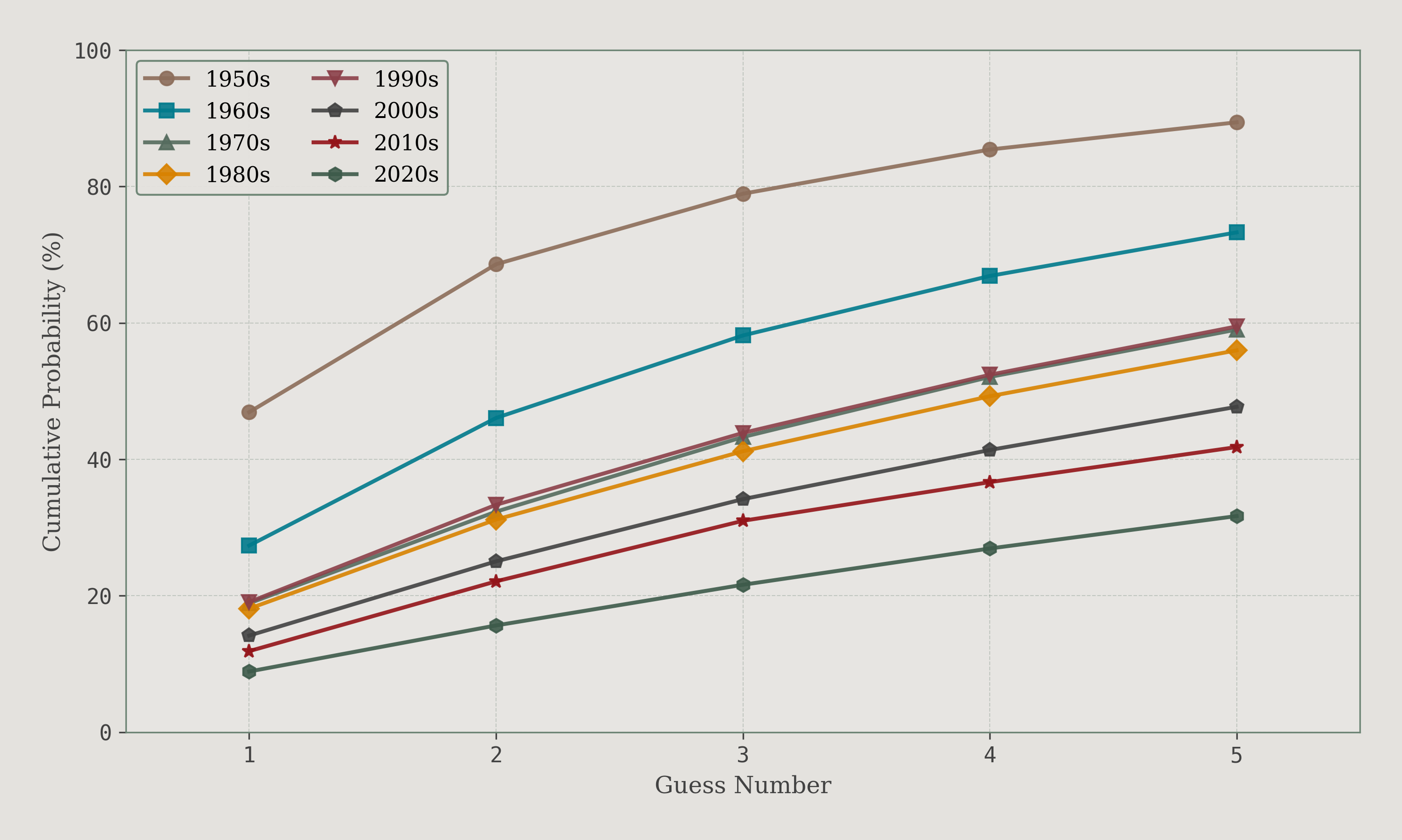
Notice how the curves change shape across decades: the 1950s curve shoots up quickly then flattens (diminishing returns), while later decades climb more steadily. This makes sense—in the smaller 1950s industry, the top guesses captured a huge proportion of connections. In today’s larger, more diverse industry, connections are spread thinner.
A single Bollywood movie, Sye Raa Narasimha Reddy, has made the list in the 2020-2024 time frame. It can be questioned how useful this guess actually is in practice if the target movie is a Hollywood production. It likely makes the list because the previous four guesses have burned so many Hollywood crew members that the most connected remaining movies are Bollywood productions.
Since the titles included were limited to having more than 2000 IMDb votes, this may impact results. I believe, however, that this is a defensible choice, since titles with fewer votes are obscure and most likely not well-connected, so they are exceedingly unlikely to be played by an opponent. I did, however, try to filter by more than 5000 votes and to my surprise, it actually made quite a difference. Most notably, the top two positions swap:
| Rank | >2000 votes | Probability | >5000 votes | Probability |
|---|---|---|---|---|
| 1 | The Player | 8.1% | Avengers: Endgame | 10.0% |
| 2 | Avengers: Endgame | 7.3% | The Player | 9.7% |
| 3 | Movie 43 | 7.1% | Movie 43 | 9.5% |
| 4 | The Dark Knight Rises | 6.8% | The Dark Knight Rises | 9.0% |
| 5 | Pearl Harbor | 6.2% | Pearl Harbor | 7.9% |
The stricter filter (>5000 votes) elevates Avengers: Endgame to the top position while demoting The Player to second. This occurs because filtering out less popular films removes many obscure titles that The Player’s cameo actors appeared in, while Avengers' connections are predominantly to well-known blockbusters that survive the stricter threshold.
The effect is even more pronounced for the 2020-2024 decade, where the bottom two positions change completely:
| Rank | >2000 votes | Probability | >5000 votes | Probability |
|---|---|---|---|---|
| 1 | Avengers: Endgame | 6.5% | Avengers: Endgame | 8.9% |
| 2 | The Dark Knight Rises | 5.6% | The Dark Knight Rises | 7.4% |
| 3 | Movie 43 | 5.2% | Movie 43 | 7.1% |
| 4 | Rogue One: A Star Wars Story | 5.2% | Zack Snyder’s Justice League | 6.8% |
| 5 | Sye Raa Narasimha Reddy | 5.1% | Spider-Man: Across the Spider-Verse | 6.5% |
The Bollywood film (Sye Raa Narasimha Reddy) disappears entirely from the top 5 with stricter filtering, replaced by more mainstream blockbusters that are far more likely to actually be played in practice.
This makes for a somewhat interesting predicament. There is no doubt that filtering by 2000 votes rather than 5000 is more “accurate”, but is that also the case in practice if 2000 vote movies are extremely unlikely to be played? We could use vote count on movies to weigh how likely it is to be played and thus optimize the guesses for this. But that creates a problem: it does not reflect individual player knowledge. The more likely a movie is to be played, the more likely the guessing player is to know a connecting movie as well, and thus not need to do optimized guessing in the first place. Such a model would need to balance movie popularity against player knowledge, which is tricky, and I am not sure such a model would be very useful if not calibrated to the individual player’s knowledge.
The limitation of vote filtering has been discussed in the previous section. Another limitation, already touched upon with regard to Bollywood movies, is that these optimized guesses are extremely Hollywood-centric. It is a common strategy for some players who are knowledgeable in a specific region’s cinema to steer their opponent into this when the opportunity presents itself, which often ends the game. The suggested guesses here, will most likely be of little help in these situations. Some of these regions occur more often than others, and a similar list could be made optimizing for most likely guesses for each, such as Scandinavian, East Asian, European, South American etc.
So what movie should you guess when completely stumped? The Player is the global optimum with an 8.1% hit rate, beating the more commonly guessed Avengers: Endgame. For decade-specific guessing, the tables above provide optimal sequences, with earlier decades showing dramatically higher success rates due to fewer total films.
One insight is that large ensemble casts don’t guarantee high connectivity, although it certainly helps. What matters more is having diverse crew members who worked across many different productions. This explains why The Player, with its smaller but well-traveled crew, outperforms bigger ensemble films.
Whether memorizing these results is worthwhile is debatable. The first 2-3 guesses probably are, but the analysis assumes uniformly random target movies. In practice, players naturally choose well-known films more often. You can’t choose a title you don’t know exists.